

'예외처리'에 해당되는 글 33건
- 2008.05.13 DSP_homework04
- 2008.05.13 DSP_homework03
- 2008.05.13 DSP_homework02
- 2008.05.13 DSP_homework01
- 2008.02.06 우사비치 4
- 2008.01.07 AVG 7.5 무료배포 이벤트!!
- 2008.01.02 만화로 보는 친일언론 현대사
- 2007.12.30 만들어진 신의 저자 "리처드 도킨스"의 인터뷰
- 2007.12.28 10대 소녀가수 '섹시' 타이틀, 타당한가?
- 2007.12.28 그림으로 보는 유쾌한 경부운하
- DSP_homework04
- 예외처리
- 2008. 5. 13. 02:12
 invalid-file
warning('off','MATLAB:dispatcher:InexactMatch')
% 4th Homework 'DFT Examples'
% (a). Find & draw |X(omega)|, |H(omega)|, |Y(omega)|
x = [ 1, 2, 2, 1];
h = [ 1, 2, 3];
y = conv (x, h);
magX1 = abs(hw4(x, length(x), 1));
magH1 = abs(hw4(h, length(h), 1));
magY1 = abs(hw4(y, length(y), 1));
figure('name', '(a) - |X(omega)|, |H(omega)|, |Y(omega)|', 'Position', [50, 350, 500, 300], 'MenuBar', 'none')
plot(magY1, 'DisplayName', 'magY1', 'YDataSource', 'magY1'); hold all; plot(magX1, 'DisplayName', 'magX1', 'YDataSource', 'magX1'); plot(magH1, 'DisplayName', 'magH1', 'YDataSource', 'magH1'); hold off; figure(gcf)
% (b) Find & draw |X(k)|, |H(k)|, |Y(k)|
x = [x, zeros(1,4)];
h = [h, zeros(1,5)];
y = [y, zeros(1,2)];
magX2 = abs(hw4(x, length(x), 2));
magH2 = abs(hw4(h, length(h), 2));
magY2 = abs(hw4(y, length(y), 2));
figure('name', '(b) - |X(k)|, |H(k)|, |Y(k)|', 'Position', [100, 300, 500, 300], 'MenuBar', 'none')
plot(magY2, 'DisplayName', 'magY2', 'YDataSource', 'magY2'); hold all; plot(magX2, 'DisplayName', 'magX2', 'YDataSource', 'magX2'); plot(magH2, 'DisplayName', 'magH2', 'YDataSource', 'magH2'); hold off; figure(gcf)
'예외처리' 카테고리의 다른 글
| DSP_homework03 (0) | 2008.05.13 |
|---|---|
| DSP_homework02 (0) | 2008.05.13 |
| DSP_homework01 (0) | 2008.05.13 |
- DSP_homework03
- 예외처리
- 2008. 5. 13. 00:40
warning('off','MATLAB:dispatcher:InexactMatch')
% 3rd Homework 'Chebyshev & Butterworth FILTERS'
% 1. (a) Design a analog Chebyshev LPF with the following properties :
% wc=10rad/s, Max 1dB ripple, N=4
% (b) Verify the result you obtained by drawing |H(w)|
OmegaC = 10;
Rp = 1;
N = 4;
% ep = sqrt(10^(Rp/10)-1);
cheby = mkfilter(OmegaC,N,'cheby',Rp);
[mag1, pha1] = bode(cheby);
figure('name', '#1 - Chebyshev Analog Filter', 'Position', [50, 350, 500, 300], 'MenuBar', 'none')
stem3 (mag1, 'DisplayName', 'mag1');
title('Magnitude Response')
xlabel('Analog frequency in pi units'); zlabel('|H|');
% 2. (a) According to the digital Butterworth LPF, draw |H(omega)| and
% discuss whether the spectrum meets the requirements of the problem.
%
% (b)For input x[n]=cos(pi/6*n)+cos(pi/2*n), n=0,1,…23 plot y[n], and
% |Y(omega)| and compare them with x[n] and |X(omega)| where y[n]=
% x[n]*h[n]
butterw = mkfilter(OmegaC,N,'butterw',Rp);
[mag2, pha2] = bode(butterw);
figure('name', '#2 (a) - Butterworth Digital Filter', 'Position', [100, 300, 500, 300], 'MenuBar', 'none')
stem3 (mag2, 'DisplayName', 'mag2');
title('Magnitude Response')
xlabel('Analog frequency in pi units'); zlabel('|H|');
N = 0:23;
input_x = cos(pi/6*N)+cos(pi/2*N);
[db1,mag3,pha,grd,w] = freqz_m(input_x,1);
for p= 1:52
ma2(p) = mag2(:,:,p);
mag4(p) = mag3(p) .* ma2(p);
end
figure('name', '#2 (b) y[n], |Y[omega]|', 'Position', [150, 150, 600, 400], 'MenuBar', 'none')
subplot(2,2,1); stem(input_x); hold all;
subplot(2,2,2); plot(ma2);
subplot(2,2,3); plot(mag3);
subplot(2,2,4); plot(mag4); hold off; figure(gcf)
'예외처리' 카테고리의 다른 글
| DSP_homework04 (0) | 2008.05.13 |
|---|---|
| DSP_homework02 (0) | 2008.05.13 |
| DSP_homework01 (0) | 2008.05.13 |
- DSP_homework02
- 예외처리
- 2008. 5. 13. 00:37
warning('off','MATLAB:dispatcher:InexactMatch')
% 2nd Homework 'Make some of IIR filter'
% #1
% (a)For Ex 6-1, draw |H(Ω)| and |H(Ω)| [dB]
w= 0:0.001:pi;
z= exp(j*w);
N= 0:23;
% (b) For input x[n]= cos(pi*n/6) + cos(pi*n/2) , n=0,1,2,…..23
% Draw |X(Ω)|, |Y(Ω)| where Y(Ω)= X(Ω)*H(Ω)
[A_Y, A_in_H, DB, A_H] = hw2(2, z, cos((pi/6)*N)+cos((pi/2)*N), 3142);
figure('name', '#1', 'Position', [100, 150, 800, 600], 'MenuBar', 'none')
subplot(2,2,1); plot(A_H); title('Response H(Ω)'); hold on;
subplot(2,2,2); plot(DB); title('Response in dB'); grid; ylabel('Decibels');
subplot(2,2,3); plot(A_in_H); title('Response X(Ω)');
subplot(2,2,4); plot(A_Y); title('Response Y(Ω)');
% #2
% (a)Passband centered at Ω=pi/4 with a BW of pi/40 between -3dB points
% Peak gain is unity
% Perfect rejection at Ω=0 and Ω= pi/2
% (b) For input x[n]= cos(pi*n/6) + cos(pi*n/2) , n=0,1,2,…..23
% Draw |X(Ω)|, |Y(Ω)| where Y(Ω)= X(Ω)*H(Ω)
[A_Y, A_in_H, DB, A_H] = hw2(4, z, cos((pi/6)*N)+cos((pi/2)*N), 3142);
figure('name', '#2', 'Position', [150, 100, 800, 600], 'MenuBar', 'none')
subplot(2,2,1); plot(A_H); title('Response H(Ω)'); hold on;
subplot(2,2,2); plot(DB); title('Response in dB'); grid; ylabel('Decibels');
subplot(2,2,3); plot(A_in_H); title('Response X(Ω)');
subplot(2,2,4); plot(A_Y); title('Response Y(Ω)');
% % #3
% % Ex 6-2 draw |H1(Ω)|, |H2(Ω)|, |H(Ω)|
H1= 1./(z.^2-1.9476.*z*cos(pi/10)+0.9483);
H2= z.^2-2.*z*cos(pi/10)+1;
H3= H1.*H2;
figure('name', '#3 |H1(Ω)|, |H2(Ω)|, |H(Ω)|', 'Position', [200, 50, 800, 600], 'MenuBar', 'none')
subplot(2,2,1); plot(abs(H1)); title('Response H1(Ω)'); hold on;
subplot(2,2,2); plot(abs(H2)); title('Response H2(Ω)');
subplot(2,1,2); plot(abs(H3)); title('Response H(Ω)');
'예외처리' 카테고리의 다른 글
| DSP_homework03 (0) | 2008.05.13 |
|---|---|
| DSP_homework01 (0) | 2008.05.13 |
| 우사비치 (4) | 2008.02.06 |
- DSP_homework01
- 예외처리
- 2008. 5. 13. 00:34
warning('off','MATLAB:dispatcher:InexactMatch')
% 1st Homework 'Using Window method'
% #1 For omega1 = pi / 2 and M = 10,
M=21;
n=-10:1:10;
wc=pi/2;
hd=ideal_lp(wc, M);
% (a) Draw w[n], W[omega] => dB scale , h[n], H[omega] in case of rect window
figure('name', 'Rectangular Window @ M=10', 'Position', [50, 420, 550, 300], 'MenuBar', 'none')
w_rect=(rectwin(M));
h=hd.* w_rect';
[db,mag,pha,grd,w] = freqz_m(h,1);
[db2,mag,pha,grd,w] = freqz_m(w_rect,1);
subplot(1,2,1); stem(n,w_rect, 'r');title('Response'); hold on; axis([-(M-8) M-8 -0.2 1.1]); xlabel('n'); ylabel('w(n)');
subplot(1,2,1); stem( n,h);
subplot(1,2,2); plot(w/pi,db2, 'r');title('Magnitude Response in dB');grid ; xlabel('frequency in pi units'); ylabel('Decibels'); hold on;
subplot(1,2,2); plot(w/pi,db); h = legend('W[Ω]','H[Ω]',1); set(h,'Interpreter','none')
% (b) Draw w[n], W[omega] => dB scale , h[n], H[omega] in case of tri window
figure('name', 'Triangular Window @ M=10', 'Position', [250, 370, 550, 300], 'MenuBar', 'none')
w_rect=(triang(M));
h=hd.* w_rect';
[db,mag,pha,grd,w] = freqz_m(h,1);
[db2,mag,pha,grd,w] = freqz_m(w_rect,1);
subplot(1,2,1); stem(n,w_rect, 'r');title('Response'); hold on; axis([-(M-8) M-8 -0.2 1.1]); xlabel('n'); ylabel('w(n)');
subplot(1,2,1); stem( n,h);
subplot(1,2,2); plot(w/pi,db2, 'r');title('Magnitude Response in dB');grid ; xlabel('frequency in pi units'); ylabel('Decibels'); hold on;
subplot(1,2,2); plot(w/pi,db); h = legend('W[Ω]','H[Ω]',1); set(h,'Interpreter','none')
% (c) Draw w[n], W[omega] => dB scale , h[n], H[omega] in case of hann window
figure('name', 'Hanning Window @ M=10', 'Position', [450, 330, 550, 300], 'MenuBar', 'none')
w_rect=(hann(M));
h=hd.* w_rect';
[db,mag,pha,grd,w] = freqz_m(h,1);
[db2,mag,pha,grd,w] = freqz_m(w_rect,1);
subplot(1,2,1); stem(n,w_rect, 'r');title('Response'); hold on; axis([-(M-8) M-8 -0.2 1.1]); xlabel('n'); ylabel('w(n)');
subplot(1,2,1); stem( n,h);
subplot(1,2,2); plot(w/pi,db2, 'r');title('Magnitude Response in dB');grid ; xlabel('frequency in pi units'); ylabel('Decibels'); hold on;
subplot(1,2,2); plot(w/pi,db); h = legend('W[Ω]','H[Ω]',1); set(h,'Interpreter','none')
% (d) Draw w[n], W[omega] => dB scale , h[n], H[omega] in case of hamming window
figure('name', 'Hamming Window @ M=10', 'Position', [650, 280, 550, 300], 'MenuBar', 'none')
w_rect=(hamming(M));
h=hd.* w_rect';
[db,mag,pha,grd,w] = freqz_m(h,1);
[db2,mag,pha,grd,w] = freqz_m(w_rect,1);
subplot(1,2,1); stem(n,w_rect, 'r');title('Response'); hold on; axis([-(M-8) M-8 -0.2 1.1]); xlabel('n'); ylabel('w(n)');
subplot(1,2,1); stem( n,h)
subplot(1,2,2); plot(w/pi,db2, 'r');title('Magnitude Response in dB');grid ; xlabel('frequency in pi units'); ylabel('Decibels'); hold on;
subplot(1,2,2); plot(w/pi,db); h = legend('W[Ω]','H[Ω]',1); set(h,'Interpreter','none')
% (e) Discuss the results
% #2 For omega1 = pi / 2 and M = 20,
M=41;
n=-20:1:20;
wc=pi/2;
hd=ideal_lp(wc, M);
% (a) Draw w[n], W[omega] => dB scale , h[n], H[omega] in case of rect window
figure('name', 'Rectangular Window @ M=20', 'Position', [50, 300, 550, 300], 'MenuBar', 'none')
w_rect=(rectwin(M));
h=hd.* w_rect';
[db,mag,pha,grd,w] = freqz_m(h,1);
[db2,mag,pha,grd,w] = freqz_m(w_rect,1);
subplot(1,2,1); stem(n,w_rect, 'r');title('Response'); hold on; axis([-(M-18) M-18 -0.2 1.1]); xlabel('n'); ylabel('w(n)');
subplot(1,2,1); stem( n,h);
subplot(1,2,2); plot(w/pi,db2, 'r');title('Magnitude Response in dB');grid ; xlabel('frequency in pi units'); ylabel('Decibels'); hold on;
subplot(1,2,2); plot(w/pi,db); h = legend('W[Ω]','H[Ω]',1); set(h,'Interpreter','none')
% (b) Draw w[n], W[omega] => dB scale , h[n], H[omega] in case of tri window
figure('name', 'Triangular Window @ M=20', 'Position', [250, 250, 550, 300], 'MenuBar', 'none')
w_rect=(triang(M));
h=hd.* w_rect';
[db,mag,pha,grd,w] = freqz_m(h,1);
[db2,mag,pha,grd,w] = freqz_m(w_rect,1);
subplot(1,2,1); stem(n,w_rect, 'r');title('Response'); hold on; axis([-(M-18) M-18 -0.2 1.1]); xlabel('n'); ylabel('w(n)');
subplot(1,2,1); stem( n,h);
subplot(1,2,2); plot(w/pi,db2, 'r');title('Magnitude Response in dB');grid ; xlabel('frequency in pi units'); ylabel('Decibels'); hold on;
subplot(1,2,2); plot(w/pi,db); h = legend('W[Ω]','H[Ω]',1); set(h,'Interpreter','none')
% (c) Draw w[n], W[omega] => dB scale , h[n], H[omega] in case of hann window
figure('name', 'Hanning Window @ M=20', 'Position', [450, 200, 550, 300], 'MenuBar', 'none')
w_rect=(hann(M));
h=hd.* w_rect';
[db,mag,pha,grd,w] = freqz_m(h,1);
[db2,mag,pha,grd,w] = freqz_m(w_rect,1);
subplot(1,2,1); stem(n,w_rect, 'r');title('Response'); hold on; axis([-(M-18) M-18 -0.2 1.1]); xlabel('n'); ylabel('w(n)');
subplot(1,2,1); stem(n,h);
subplot(1,2,2); plot(w/pi,db2, 'r');title('Magnitude Response in dB');grid ; xlabel('frequency in pi units'); ylabel('Decibels'); hold on;
subplot(1,2,2); plot(w/pi,db); h = legend('W[Ω]','H[Ω]',1); set(h,'Interpreter','none')
% (d) Draw w[n], W[omega] => dB scale , h[n], H[omega] in case of hamming window
figure('name', 'Hamming Window @ M=20', 'Position', [650, 150, 550, 300], 'MenuBar', 'none')
w_rect=(hamming(M));
h=hd.* w_rect';
[db2,mag,pha,grd,w] = freqz_m(w_rect,1);
[db,mag,pha,grd,w] = freqz_m(h,1);
subplot(1,2,1); stem(n,w_rect, 'r');title('Response'); hold on; axis([-(M-18) M-18 -0.2 1.1]); xlabel('n'); ylabel('w(n)');
subplot(1,2,1); stem( n,h)
subplot(1,2,2); plot(w/pi,db2, 'r');title('Magnitude Response in dB');grid ; xlabel('frequency in pi units'); ylabel('Decibels'); hold on;
subplot(1,2,2); plot(w/pi,db); h = legend('W[Ω]','H[Ω]',1); set(h,'Interpreter','none')
% (e) Discuss the results
% #3 For input x[n]=cos(pi/6*n)+cos(pi/2*n),
% n=0, 1, ... , 23
M=24;
N=0:M-1;
input_n= cos((pi/6)*N)+cos((pi/2)*N);
% draw X(omega) and Y(omega) where Y(omega) = X(omega)H(omega)
[db1,mag1,pha,grd,w] = freqz_m(input_n,1);
[db2,mag2,pha,grd,w] = freqz_m(hamming(M),1);
mag3 = mag1 .* mag;
figure('name', 'cos((pi/6)*N)+cos((pi/2)*N) & n=0~23', 'Position', [300, 50, 600, 250], 'MenuBar', 'none')
plot(mag3); hold all; plot (mag); plot (mag1); hold off; figure(gcf)
h = legend('Y[Ω]','X[Ω]','H[Ω]',0); set(h,'Interpreter','none'); axis([0 500 0 24]);
'예외처리' 카테고리의 다른 글
| DSP_homework02 (0) | 2008.05.13 |
|---|---|
| 우사비치 (4) | 2008.02.06 |
| AVG 7.5 무료배포 이벤트!! (0) | 2008.01.07 |
문제가 있다면 삭제하겠습니다.
1 식사의 시간 2 노동의 시간 3 샤워의 시간 4 오락의 시간 5 댄스의 시간
6 면회의 시간 7 체조의 시간 8 도박의 시간 9 간식의 시간 10화장실의 시간
11 처형의 시간 12 린치의 시간 13 출소의 시간 [시즌 1 끝] 14 난폭운전주의 15 한눈팔기운전주의
16 비탈길발진주의 17 저격주의 18 댄스주의 19 미사일주의 20 펑크주의
21 과속주의 22 전차주의 23 개조주의 24 위장주의 25 검문주의 26 총공격주의 [시즌 2 끝]
'예외처리' 카테고리의 다른 글
| DSP_homework01 (0) | 2008.05.13 |
|---|---|
| AVG 7.5 무료배포 이벤트!! (0) | 2008.01.07 |
| 고뉴스 라이브채팅 [원더걸스]편 (7) | 2007.11.21 |
- AVG 7.5 무료배포 이벤트!!
- 예외처리
- 2008. 1. 7. 05:01
행사는 Computeract! 라는 잡지에서 라고합니다.
다운로드
자세한 정보를 원하시는 분은 http://skysummer.com/470 로 고고
30달러(영국)짜리 정품이라고 합니다.
요세 안티바이러스 고민이시죠?
1년간 무료랍니다.
무료라면 굼벵이도 먹는다고합니다.
무엇이 고민이십니까?
일단 설치하고 봅니다.
아멘!
'예외처리' 카테고리의 다른 글
| 우사비치 (4) | 2008.02.06 |
|---|---|
| 고뉴스 라이브채팅 [원더걸스]편 (7) | 2007.11.21 |
| 난투 (0) | 2007.10.27 |
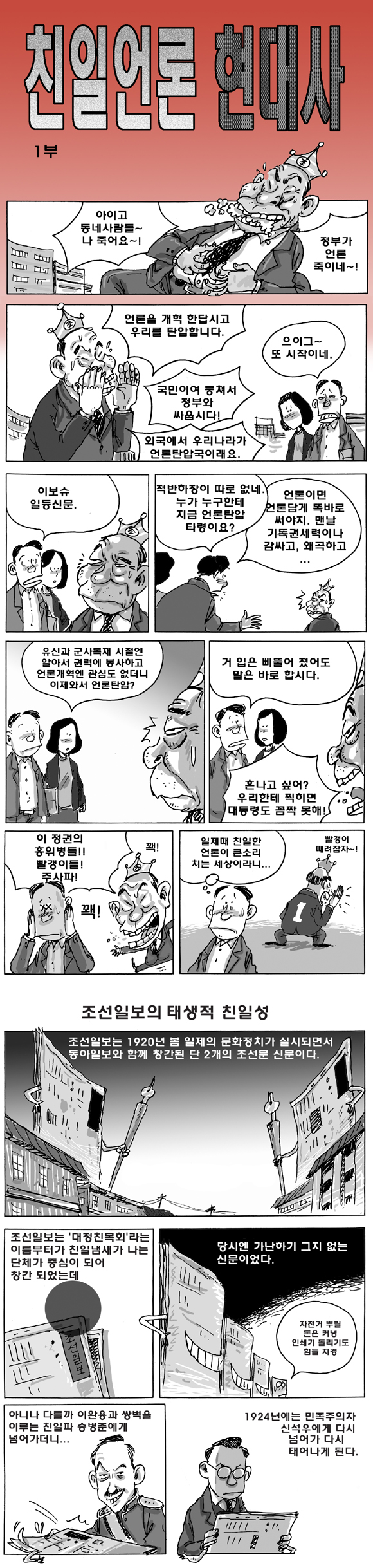
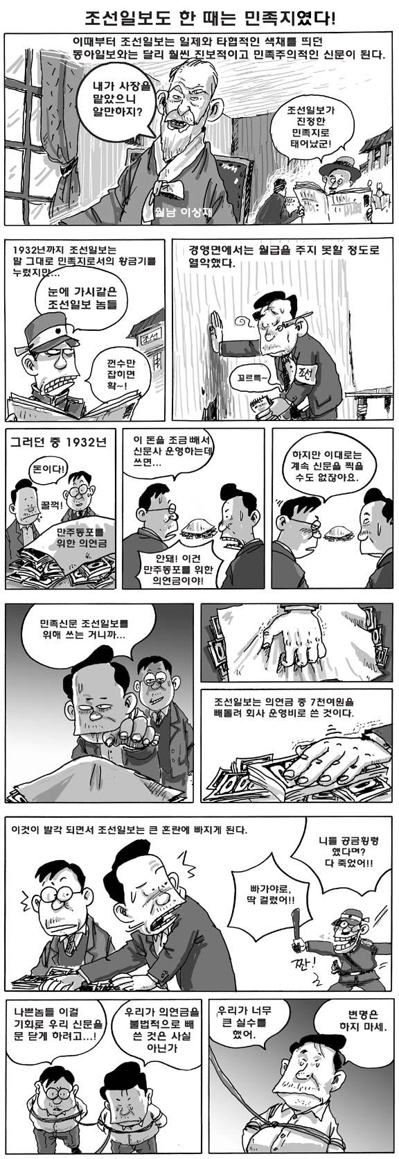
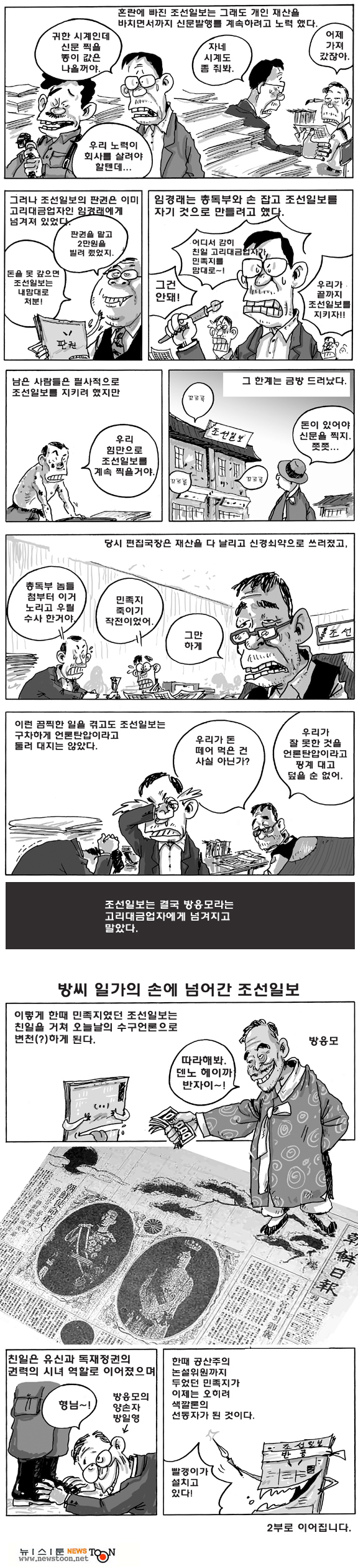
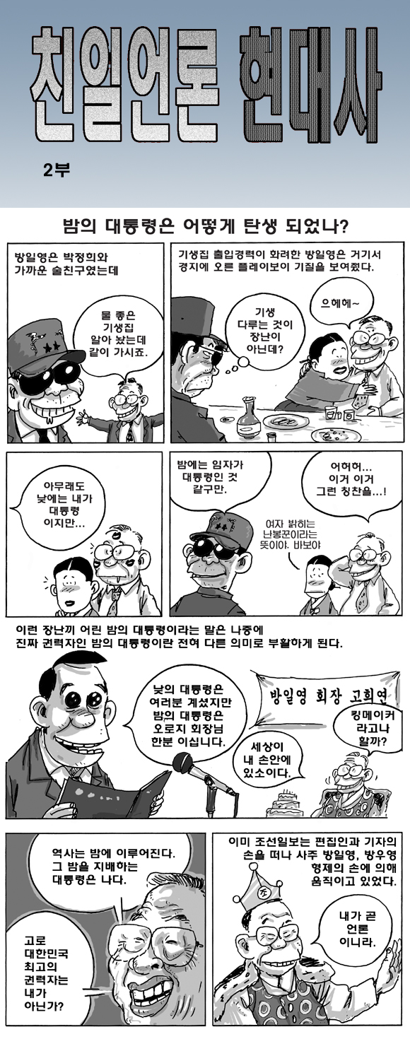
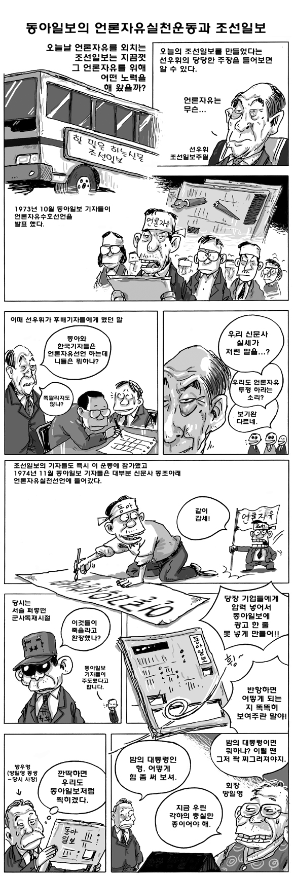
- 만화로 보는 친일언론 현대사
- 예외처리/개념탑제하기
- 2008. 1. 2. 04:38
출처 : 그림에 표기되어 있음
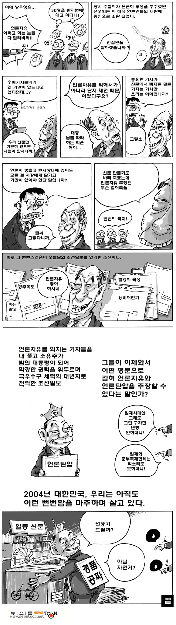
출처 : 그림에 표기되어 있음
'예외처리 > 개념탑제하기' 카테고리의 다른 글
| 커피 이름 (0) | 2008.11.24 |
|---|---|
| 만들어진 신의 저자 "리처드 도킨스"의 인터뷰 (0) | 2007.12.30 |
| 10대 소녀가수 '섹시' 타이틀, 타당한가? (0) | 2007.12.28 |
- 만들어진 신의 저자 "리처드 도킨스"의 인터뷰
- 예외처리/개념탑제하기
- 2007. 12. 30. 12:28
개념충만을 넘어서 포화상태인 이 사람
책을 읽어볼까?
'예외처리 > 개념탑제하기' 카테고리의 다른 글
| 만화로 보는 친일언론 현대사 (0) | 2008.01.02 |
|---|---|
| 10대 소녀가수 '섹시' 타이틀, 타당한가? (0) | 2007.12.28 |
| 그림으로 보는 유쾌한 경부운하 (0) | 2007.12.28 |
- 10대 소녀가수 '섹시' 타이틀, 타당한가?
- 예외처리/개념탑제하기
- 2007. 12. 28. 15:31
이거 내가 진작부터 얘기하고 싶었다.
언제부터인가 "Sexy"라는 말을 입에 달고 사는 TV를 보고 있자니 한숨이 나왔다.
10대 소녀가수뿐만이 아니다.
신동 [神童] 을 대상으로 하는 프로그램에도 항상 뒤따른다.
미처 10세가 되지 않은 꼬마여자아이들도 방송에는 'Sexydance'라며 좋은 의미인 양 추켜세우는 경우도 허다하다.
이는 과다한 외래어 남용에도 그 이유가 있는 것이다.
이 기사와 일맥상통까지는 아니더라도 비슷한 내용의 기사라니 속이 시원한 느낌이 든다.
'예외처리 > 개념탑제하기' 카테고리의 다른 글
| 만들어진 신의 저자 "리처드 도킨스"의 인터뷰 (0) | 2007.12.30 |
|---|---|
| 그림으로 보는 유쾌한 경부운하 (0) | 2007.12.28 |
| 정의는 없다. (0) | 2007.12.25 |
- 그림으로 보는 유쾌한 경부운하
- 예외처리/개념탑제하기
- 2007. 12. 28. 01:20
글쓴이 : 운하
원본 링크 : http://www.seoprise.com/board/view.php?table=seoprise_10&uid=192777
그림으로 보는 유쾌한 경부운하
MB가 당선된 이상, 뭐라고 떠들어봐야 대세는 MB인 거고, 그래서 지금 최고 이슈가 되고 있는 게 경부운하인데…
많은 분들이 식수원이고 하상계수고 관광자원이고 이익창출효과 세금낭비 공사기간 등등을 문제 삼아 열 올리는 거 알고 있어. 세상에 정말 똑똑한 사람이 많구나 하고 감탄중이야.
그래서 글재주가 별로 없는 나는 아주 아주 단순하고 원론적인 문제를 그림으로 다 함께 즐겨보고 싶어졌어. (말투가 Dc냄새가 나는 건 미안해. 하지만, 딱딱하게 썼다간 포스팅하던 나부터 스트레스를 받을 것 같아 나름 분위기를 누그러뜨리고 싶었어. 반말이 기분 나쁜 분 계시면 먼저 사과할게.)
일단 MB께서 모델로 삼고 계시는 독일의 지리를 좀 보자고
 |
대략 이 근처 물길이 이런 구조야. 엉성해서 미안하지만 그냥 느낌만 봐. 네덜란드는 매립지와 운하에 목숨 거는 나라니 벌집이 따로 없어.
일단은 제일 눈에 들어오는 게 킬(kiel)운하.
주전자 손잡이처럼 어정쩡하게 튀어나온 덴마크가 얄미워서라도 누구든 뚫고 싶었을 거야.
북해에서 발트해를 빙 둘러가는 게 얼마나 짜증나는지는 '대항해시대'를 해본 사람은 잘 알겠지. 목재 팔러 런던-오슬로 앵벌이 하던 생각이 무럭무럭 나네…
뭐가 됐건 아우토반까지 해서, 독일은 전쟁 많이 해본 나라답게 수송수단 확보에 열과 성을 다했지. 킬 운하도 군함들이 룰루랄라 잘들 애용하던 길이라더군.
아무튼 보다시피 독일은 바다에 접한 지역이 별로 없어. 그리고 한가지 알게 된 사실은 이 물길이 내륙용만은 아니더라는 거야. 특히나 라인-마인-도나우강은 네덜란드에서 흑해까지 연결되는 물길의 연장선이더라고.
아래 그림을 보면 알 수 있을 거야. 그리고 세계적으로도 유명한 파나마, 수에즈 운하를 보자고.
 |
길게 설명할 거 없이,
위의 그림들만 봐도 운하를 짓게 되는 이유는 이거 하나야. (글의 오류를 지적하는 분이 나오셔서 추가하는데, '바다로 둘러싸인 동네에서 운하를 짓게 되는 이유'라고 덧달게)
 |
돌아가는 짓을 못 해먹겠으니 질러가잔 거야. 다시 말해 '지름길 확보'를 위한 것이지. 결과적으로 얻게 되는 게 시간절약 물자절약이고.
자, 이제
it's show time이야.
함께 웃어보자고.
 |
난 뭐, 다 필요 없고 이 그림 하나만으로도 웃겨서 살 수가 없어. 어떻게 가로도 아니고 세로로 라인이 나오지? 심지어 주변은 물 천지야.
조금 더 웃어볼까?
우리나라 산맥 어떻게 뻗어있는지 기억하는 사람?
 |
명박 어린이, 지리 시간에 자느라 수고하셨쎄요. 정말이지 새삼 의무교육의 소중함을 느껴.
이게 무슨 천로역정도 아니고 뛰어갈 길을 기어가는 것도 모자라 산을 뚫고 있냐?
난 명박이한테 심시티보다는 대항해시대를 선물해야 한다고 봐. 그리고 누가 그렌라간 좀 그만 보라고 해줘. 제발….
p.s
'운하'의 정의 자체부터 무시하고 말도 안 되는 라인을 잡고 있는다. 이 말은 결국 운하가 지나가는 지역의 땅값 올리기나 건설업체와 쿵작작… 이게 본심이란 소리야.
운하가 필요하기 때문에 짓는 게 아니라는 말이야. 거기에 이유를 갖다대려니 억지춘향이 난무하는 거고.
이건 개념 없고 상식이 없어서 밀어붙이는 게 아니야. 그래서 아무리 논리정연한 이유로 반박한들 소용이 없는 거야.
개그하다 막판에 슬퍼지네.
원본 출처 : 서프라이즈
글쓴이 : 운하
원본 링크 : http://www.seoprise.com/board/view.php?table=seoprise_10&uid=192777
'예외처리 > 개념탑제하기' 카테고리의 다른 글
| 만들어진 신의 저자 "리처드 도킨스"의 인터뷰 (0) | 2007.12.30 |
|---|---|
| 10대 소녀가수 '섹시' 타이틀, 타당한가? (0) | 2007.12.28 |
| 정의는 없다. (0) | 2007.12.25 |


Recent comment